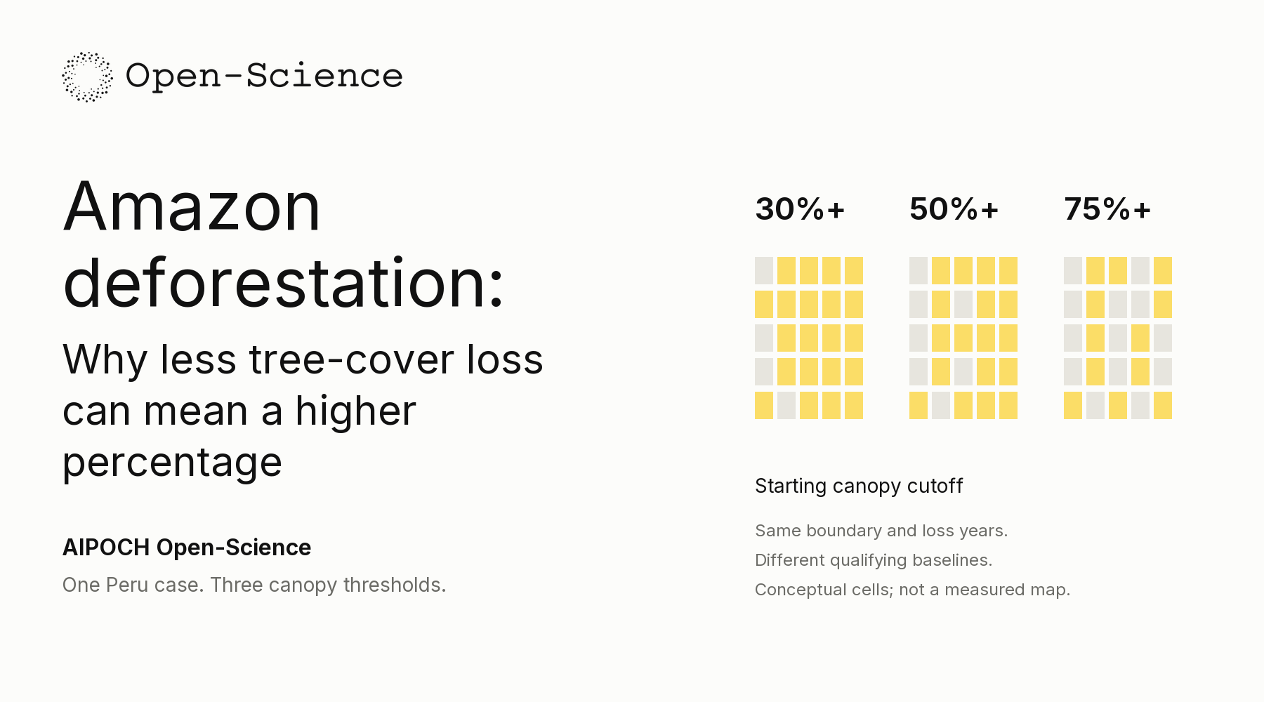
How can a stricter canopy definition produce fewer hectares of tree-cover loss but a larger loss percentage? In one fixed study box near Iberia, Peru, raising the starting canopy cutoff from 30% to 75% reduces mapped loss by 1.08%, while the share of the qualifying baseline with mapped loss rises from 55.54% to 56.61%.
The apparent contradiction is the entry point to Amazon Tree-Cover Loss — Does the Definition Change the Picture?, a public .science case in AIPOCH Open-Science. The package connects the report to saved inputs, CSV tables, code and original figures, so readers can follow the denominator behind each percentage.
Readers arriving through searches for Amazon deforestation data should keep the measured quantity in view: the case summarizes mapped tree-cover loss in a local rectangle, without independently measuring permanent land-use conversion or basin-wide deforestation.
One fixed Peru window, three starting baselines
The Iberia comparison isolates the effect of a canopy definition by applying three cutoffs to the same year-2000 tree-cover layer, fixed geographic boundary and loss-year record, allowing readers to see which pixels enter each baseline before interpreting the hectares or percentages reported for the selected area.
The AIPOCH case record (2026) fixes a 482.90 km² box near Iberia, Madre de Dios, and compares inclusive canopy cutoffs of 30%, 50% and 75%.
The GFC v1.12 layer documentation (verified 2026) defines treecover2000 as estimated canopy closure for vegetation taller than five metres and supplies encoded loss years through 2024.
The recorded analysis is dated 29 September 2026. Its boundary—69.60–69.40°W and 11.50–11.30°S—stays fixed throughout. The dataset is GFC-2024-v1.12, with complete loss years 2001–2024. The dataset's required methodological attribution is Hansen et al. (2013), High-Resolution Global Maps of 21st-Century Forest Cover Change, Science 342, 850–853.
The saved code first selects mapped land using datamask, then applies the cutoff to canopy cover in 2000. Eligible cells contribute their full area; an 80%-canopy cell is not counted as 0.8 of a cell. Loss-year codes identify which eligible cells contribute to the annual and cumulative sums.
Each input layer contains an 800 × 800 window. analyze_iberia.py weights cells by their WGS84 ellipsoidal surface area, avoiding a nominal 30 m × 30 m assumption. study_boundary.geojson records the boundary, while iberia_inputs.npz retains the arrays. Together, the files expose both the geographic selection and the rule deciding which cells count.
The denominator shrinks faster than mapped loss
The Iberia loss share rises under the stricter canopy cutoff because the eligible starting baseline shrinks faster than cumulative mapped loss, so fewer hectares in the numerator can still represent a larger fraction of the remaining denominator when the same observation years and geographic boundary are retained.
The case's saved threshold comparison (2026) reports 25,133.1 hectares of mapped loss from a 45,252.2-hectare baseline at the 30% cutoff. The same case table (2026) reports 24,860.9 hectares of loss from a 43,919.7-hectare baseline at the 75% cutoff.

Case output threshold_sensitivity_chart.png, embedded intact. GFC v1.12 processing: spatial extraction, canopy filtering, area-weighted summaries and visualization. Credit: Hansen/UMD/Google/USGS/NASA; CC BY 4.0. The outer explanation was added for this article.
| Starting canopy cutoff | Baseline area | Cumulative mapped loss | Loss / own baseline |
|---|---|---|---|
| At least 30% | 45,252.2 ha | 25,133.1 ha | 55.54% |
| At least 50% | 44,848.8 ha | 25,067.4 ha | 55.89% |
| At least 75% | 43,919.7 ha | 24,860.9 ha | 56.61% |
The calculation is:
Loss share (%) = cumulative mapped-loss area ÷ qualifying year-2000 baseline area × 100.
Raising the cutoff removes approximately 272.2 hectares of mapped loss, a 1.08% reduction, and 1,332.5 hectares of baseline area, a 2.94% reduction. The denominator contracts more proportionally, so the loss share increases by approximately 1.07 percentage points. A percentage-point change describes the difference between two shares; the relative area reduction answers a different question.
canopy_band_summary.csv makes the change tangible: the 30–<50% band contributes about 65.65 hectares of mapped loss, and the 50–<75% band about 206.53 hectares. Most mapped loss in the comparison lies in cells with high starting canopy, explaining why the hectare totals remain close.
The denominator is fixed through time within each threshold's series, but differs between thresholds. The three choices therefore test sensitivity to a definition. The comparison does not identify a universally correct forest cutoff or predict how sensitive a more sparsely wooded landscape would be.
A persistent peak, with limits on interpretation
The Iberia record keeps a pronounced 2024 mapped-loss peak under every tested canopy cutoff, showing that the temporal pattern survives the definition change within the selected box while leaving disturbance causes, permanent land-use change and classification accuracy unresolved without independent evidence beyond the saved maps and summaries.
The case's annual results (2026) report 6,731.6 hectares of mapped loss in 2024 at the 30% cutoff and 6,687.0 hectares at 75%. The GFC v1.12 usage notes (verified 2026) caution about temporal inconsistencies and advise against definitive area estimation by simply counting mapped loss pixels.
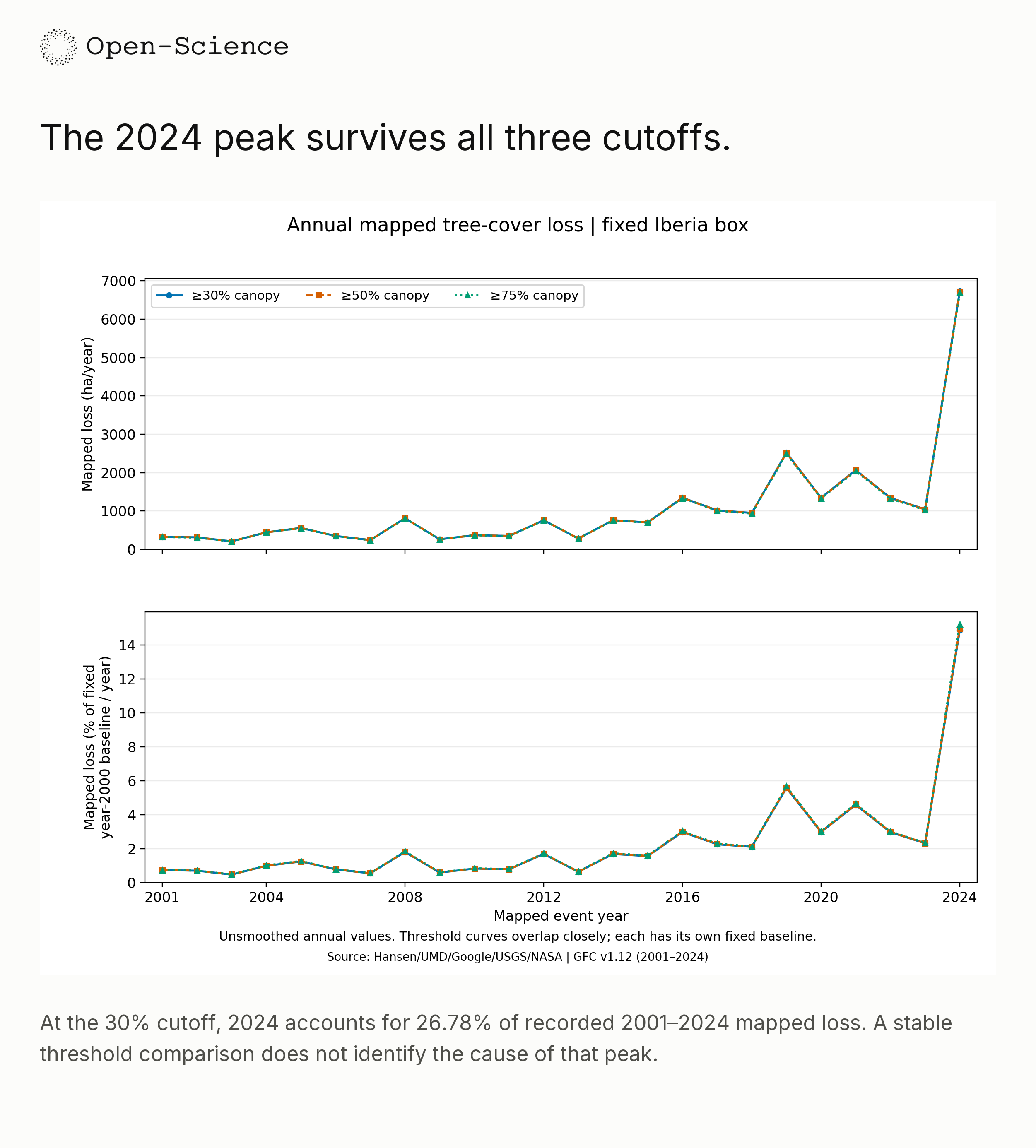
Case output annual_loss_chart.png, embedded intact. GFC v1.12 processing: spatial extraction, canopy filtering, area-weighted summaries and visualization. Credit: Hansen/UMD/Google/USGS/NASA; CC BY 4.0. Lower-panel percentages use each threshold's own fixed baseline.
At 30%, the 2024 total is about 6.43 times the 2023 total and contributes 26.78% of all mapped loss in 2001–2024. The unmodified annual chart preserves the earlier increases and declines, keeping the peak in context.
Period comparison: period_summary.csv records mean annual mapped loss of 417.7 ha/year for 2001–2012 and 1,676.7 ha/year for 2013–2024; excluding the peak leaves 1,217.2 ha/year for 2013–2023. The summaries are descriptive. The 2013 division coincides with Landsat 8 inclusion, and the release notes describe reprocessing from 2011 onward and Landsat 9 inclusion from 2022, limiting a literal before/after interpretation.

Case output loss_timing_map.png, embedded intact. GFC v1.12 processing: spatial extraction, canopy filtering, area-weighted summaries and visualization. Credit: Hansen/UMD/Google/USGS/NASA; CC BY 4.0. “No mapped loss” does not establish undisturbed forest.
The maps help locate the recorded pattern, but no independent fire, roads, land-use or other causal layers were overlaid. A mapped stand-replacement event can reflect clearing, harvesting, fire or another qualifying disturbance; assigning a cause or establishing permanence needs additional evidence.
The small threshold spread is also not a confidence interval. Different cutoffs expose definition sensitivity, without measuring missed events, false detections or timing errors. Area weighting improves geometry, while independent reference interpretation and an appropriate sampling design are needed to assess classification and derive accuracy-adjusted area estimates.
Trace the loss share through the .science package
The Iberia package offers a concrete reading path from a loss percentage to the corresponding baseline row, calculation code and saved evidence, enabling readers to examine how the result was produced while keeping the sender's recorded reproducibility checks separate from any new execution or validation on a receiving computer.
The case's archived materials (2026) include the report, threshold_summary.csv, canopy_band_summary.csv, analyze_iberia.py and verification.json.
The official .science guide (verified 2026) describes read-only imported history and desktop Fork support from v0.31.0, with a compatible reader required for the package format.
Begin with one question: why does 56.61% exceed 55.54% when loss hectares decrease? Open iberia_tree_cover_loss_report.md, then compare baseline_ha, mapped_loss_ha and loss_pct_baseline in threshold_summary.csv. The formula above should connect the table columns directly.
Inspect analyze_iberia.py for the land mask, inclusive canopy cutoff, encoded loss-year filter and area weights. Follow canopy_band_summary.csv to the contribution removed by each tighter definition. The sequence turns a chart's percentage into an inspectable choice about which cells qualify.
verification.json records the sender's fresh-process input reconstruction, byte-identical CSV outputs and pixel-identical PNG outputs. For this article, the complete package, selected report and tables, relevant calculation code and three original figures were checked statically; the archived research scripts were not executed. Computational agreement does not independently validate the satellite classifications.
To explore the record, download the package from the case page, use the project's import flow, review the target and contents, and wait for completion. For new work, use Fork in desktop v0.31.0 or later, with a compatible reader. This package declares the ro-crate capability, for which the guide specifies v0.33.0 or a later compatible reader. Fork does not automatically execute code or restore credentials.
Does 55.54% describe the whole Amazon?
No. The share uses the qualifying year-2000 baseline inside the fixed Iberia box. The box is a local case rather than a representative regional sample, and the mapped loss measure does not independently establish permanent deforestation.
Does subtracting cumulative loss give current forest area?
No. Baseline minus encoded loss gives the starting area without a recorded loss event. Regrowth, later disturbances and initially sparse vegetation are not fully represented in that subtraction.
Open the Iberia case and explore its .science package, starting with the two denominators behind 55.54% and 56.