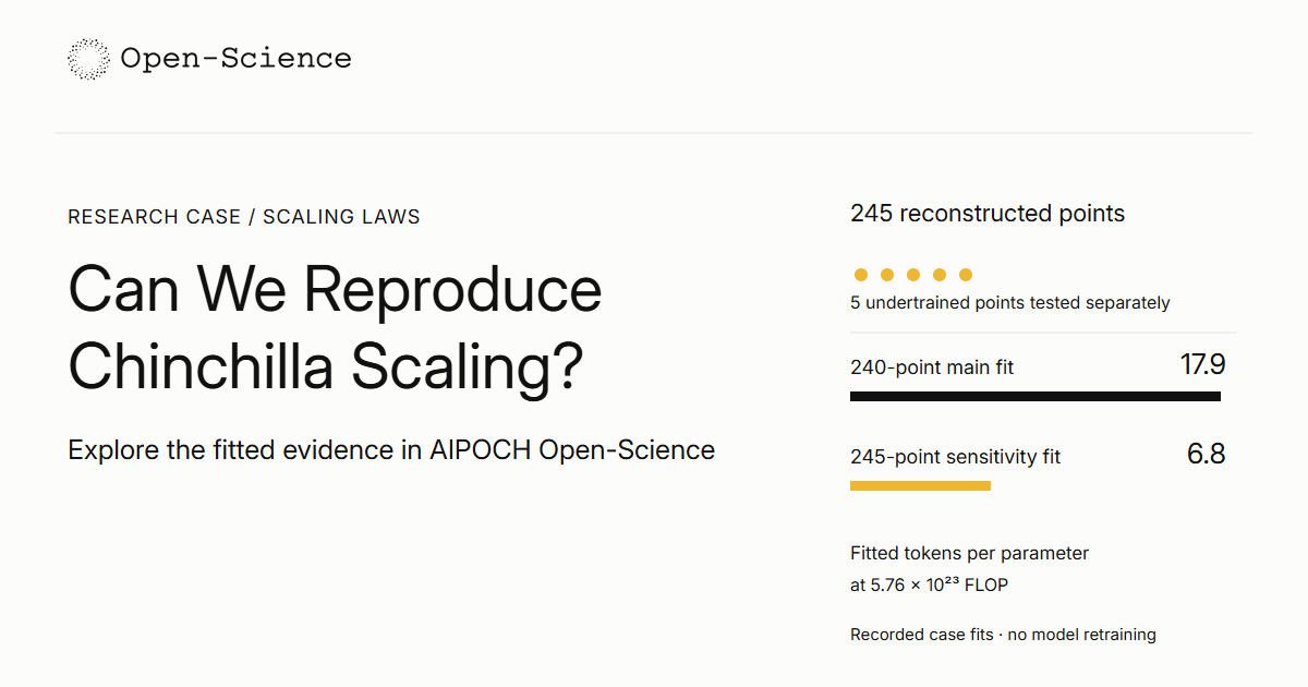
At Chinchilla’s training budget, how many tokens should a model see per parameter? A refit of 240 observations gives 17.9. Put five observations back and the estimate falls to 6.8, at exactly the same budget. Both numbers come from the same figure and the same equation.
The AIPOCH Open-Science .science package lets a reader trace that difference from the plotted observations through the fitted coefficients to the allocation table. It also preserves two sets of bootstrap results that explain how a fit can look far more precise than the data warrant. The case refits published measurements. Its evidence concerns a scaling law, while Chinchilla’s training run and downstream performance are separate experiments. Open the public case and its package.
How closely does the refit match?
On the same 240 observations, the AIPOCH Open-Science refit and the Epoch AI replication predict training loss with almost identical error, while the coefficients printed in the original paper tend to predict too much loss, particularly for models trained on relatively few tokens per parameter.
Approach 3 estimates final loss from model size and training tokens, one of three ways the original authors studied compute allocation in Hoffmann and colleagues’ 2022 paper. Epoch AI reconstructed 245 observations from Figure 4 and set aside the five with the highest losses in its main analysis, a choice documented in the 2024 replication, version 2.
The model is L(N, D) = E + A/N^α + B/D^β. Here N counts model parameters, D counts training tokens, and E is the fitted limiting loss. The case derives token counts from compute using D ≈ C/(6N). That makes the 245 rows a reconstruction of a published figure, with token counts inferred from an approximation. The original training dataset contains more information than the plot preserves.
For its main fit, the case searches 4,500 starting combinations and retains the lowest sum of Huber penalties on log-loss residuals (δ = 0.001). A positive raw residual means predicted loss exceeded observed loss. Scored on the same rows, the three fits give the following results.
| On the 240 main observations | Printed 2022 coefficients, rounded | Epoch AI fit | Case refit |
|---|---|---|---|
| Token exponent β | 0.28 | 0.3658 | 0.3672 |
| Sum of log-space Huber penalties | 0.00412 | 0.00102 | 0.00102 |
| Raw-loss RMSE | 0.0526 | 0.0218 | 0.0218 |
| Mean predicted minus observed loss | +0.0447 | −0.0008 | −0.0021 |
The roughly fourfold Huber gap compares the rounded, printed coefficients with the case refit. Epoch AI also tested the higher-precision coefficients in the original paper’s TeX source. Those closed most of the fit gap in its comparison, although a discrepancy remained. The fourfold figure therefore measures the combined discrepancy for the printed values. It cannot isolate an optimizer effect. Replication, §3.1.
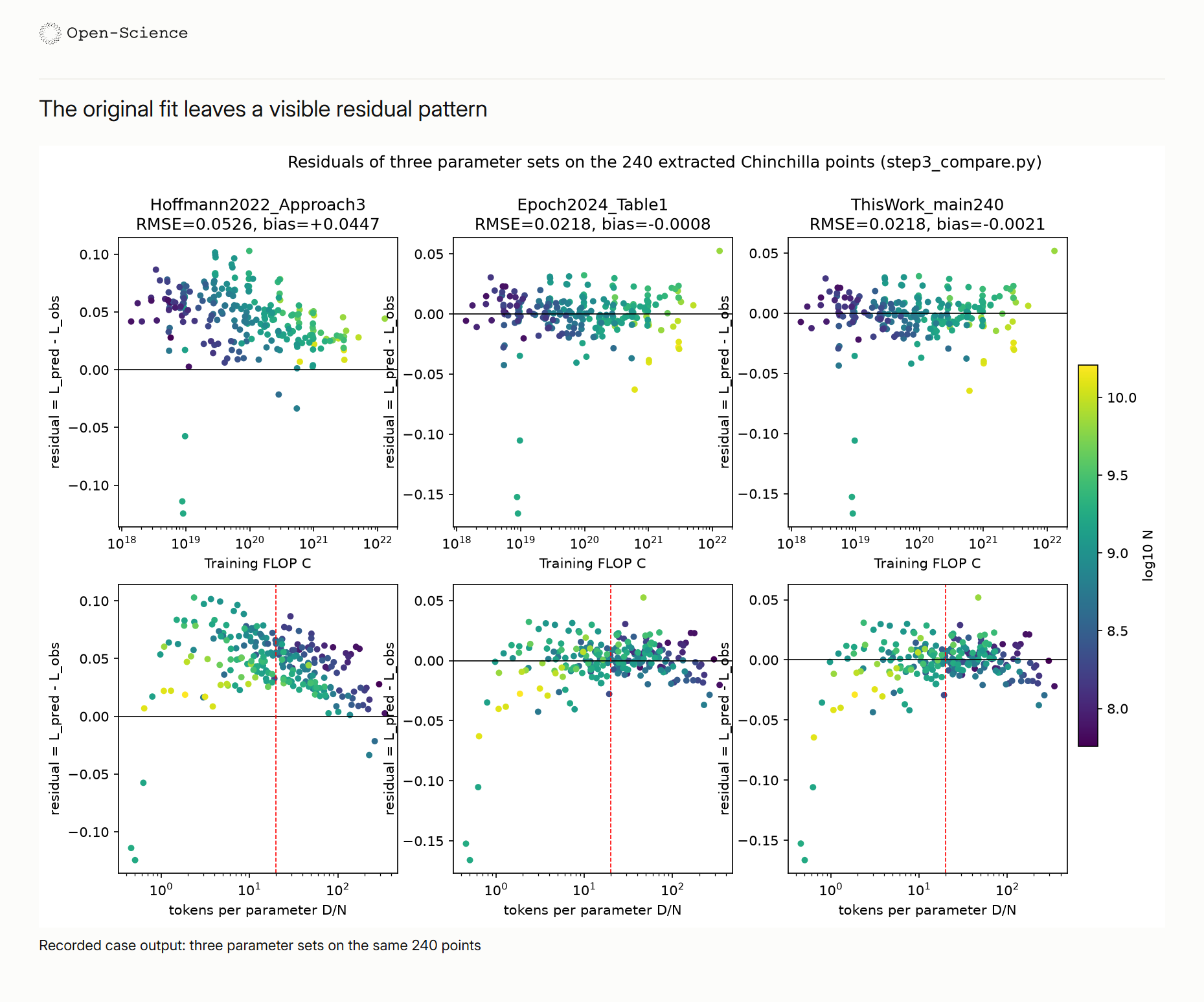
Read the lower row from left to right. The rounded coefficients systematically overpredict loss across part of the tokens-per-parameter range. The two refits reduce that pattern. All three panels show in-sample errors.
Why does the uncertainty interval change?
Across the same 500 bootstrap resamples, the estimated model-size exponent varies about 35 times as much when the optimizer uses tighter stopping criteria and an analytic gradient, even though both runs start from the same full-sample solution and see exactly the same observations on every draw.
Averaging Huber penalties instead of summing them changed the objective’s scale and triggered early stopping in the original optimization, according to the original authors’ explanation reported in the 2024 replication, §3.1. The paired comparison in the 2026 AIPOCH Open-Science case tests the effect of changing both stopping criteria and gradient calculation in its own implementation.
The exponent a = β/(α + β) describes how optimal model size grows as compute increases. Its estimate from the full 240-row fit is 0.5139. Each bootstrap fit starts from the full-sample fitted coefficients, without repeating the 4,500-start search. If the optimizer stops close to its starting point on every draw, different resamples can yield nearly identical estimates.
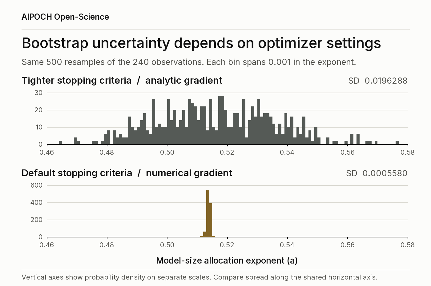
Editorial replot of the first 500 paired draws. Both panels use the same bins and horizontal scale. Their vertical density scales differ so each distribution is legible. The sample standard deviations are 0.0196288 and 0.0005580. The archived chart uses 2,000 versus 500 draws, separate bins, and raw counts. View the original case figure.
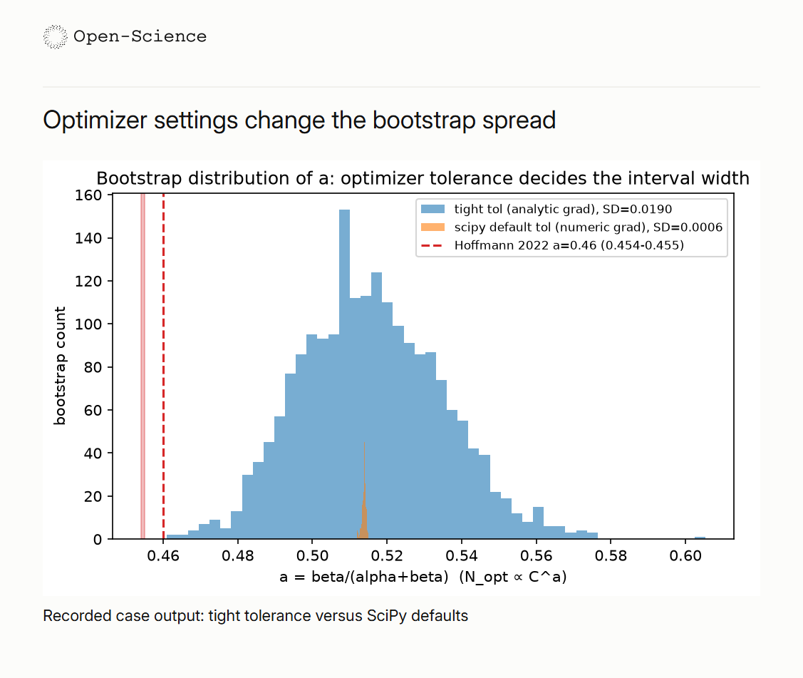
Two interval designs answer different questions. Across 2,000 draws with replacement, the tighter fit gives a 95% percentile interval of 0.4820–0.5553 for a. To compare with the original paper’s procedure, the case separately takes 100 subsamples, each containing 80% of the rows without replacement. Its 10th–90th percentile interval is 0.4993–0.5251, a width of 0.0258.
The original paper’s Table 2 prints 0.46 as the point estimate and 0.454–0.455 as its percentile range. The case also calculates a directly from the printed α and β (0.4516) and from their higher-precision values (0.4565). Each number has a different source. The narrow range belongs to Table 2’s subsampling result. Original Table 2.
What happens when the five points go back in?
Restoring five unusually undertrained models moves the projected allocation at Chinchilla’s compute budget from about eighteen tokens per parameter to about seven, because the extra observations change the fitted response to training data and the budget lies far beyond the largest run in the reconstructed sample.
The five highest-loss observations span roughly 0.036 to 0.404 tokens per parameter in the 2026 AIPOCH Open-Science case. Including all five changes the estimated scaling policy, a sensitivity also examined in Appendix A.1 of the 2024 replication.
With all 245 observations, the token exponent β rises from 0.3672 to 0.4530. On the original 240 rows, the all-points fit even has a lower raw-loss RMSE (0.0190), alongside a higher log-space Huber objective (0.00116). The fit optimized the latter measure. The five runs are informative precisely because they sample a different training regime.
| Compute budget | Main fit, tokens per parameter | Main fit, 95% interval | All 245, tokens per parameter |
|---|---|---|---|
| 10²¹ FLOP | 21.4 | 15.6–28.3 | 15.5 |
| 5.76 × 10²³ FLOP | 17.9 | 7.8–35.5 | 6.8 |
| 10²⁶ FLOP | 15.5 | 4.5–42.4 | 3.5 |
The intervals are percentile-bootstrap intervals conditional on the selected 240 observations and the fitted loss function. They omit uncertainty from digitizing the figure, choosing the functional form, and extrapolating beyond the observed budgets.
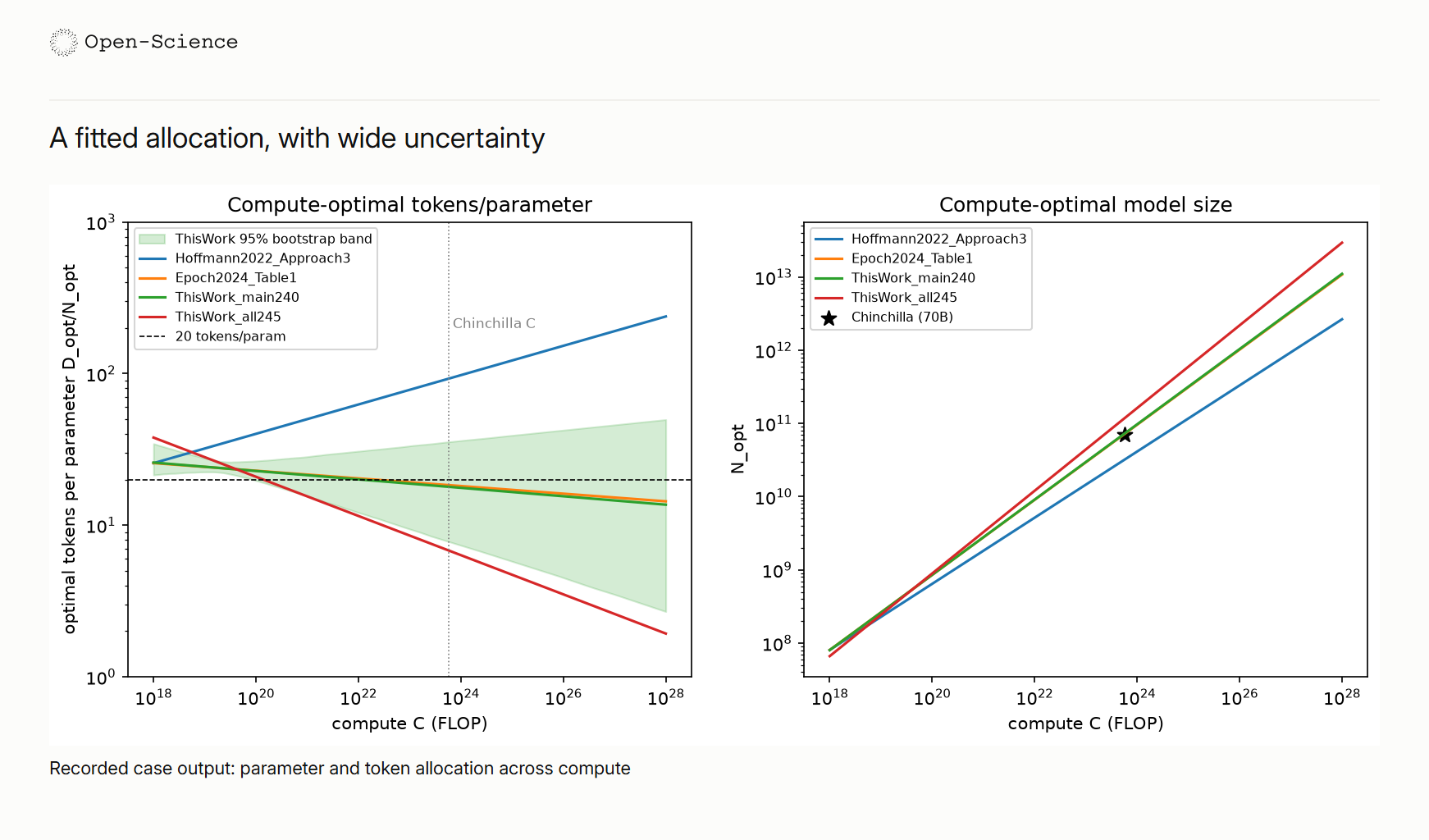
In the left panel, the vertical dotted line marks Chinchilla’s budget. It is about 44 times the largest observed budget of 1.3 × 10²² FLOP. The red and green curves show how far the two sample choices have diverged there.
The main fit gives model-size and token exponents of 0.5139 and 0.4861 as compute grows. Their difference in the order token exponent minus model-size exponent is −0.0278, with a 95% bootstrap interval from −0.1105 to +0.0360. Near-equal growth is compatible with the evidence. At Chinchilla’s budget, 20 tokens per parameter also sits inside the main interval, but the data leave room for substantially different allocations.
Follow the estimate through the package
Open REPORT.md in the public case and pick one number, 17.9. Find its row in results/step5_optimal_alloc_by_C.csv, compare the 240- and 245-row fits in results/step3_param_comparison.csv, then inspect the five observations in data/excluded_points.csv. Those three files show how an editorially simple training rule depends on a specific decision about the sample. Explore the Chinchilla case in AIPOCH Open-Science.
FAQ
Did the case independently establish why the original optimizer stopped early? The historical explanation comes from the original authors as reported by Epoch AI. The package demonstrates a related mechanism in a separate implementation. It changes both gradient calculation and stopping criteria, so their individual contributions remain unresolved. Replication, version 2.
Does importing the package run the analysis again? Import opens the selected files and read-only research record. Recalculating the results requires a deliberate new run in a writable environment. For this article, the matched standard deviations were recalculated from saved draws. The model fits and training runs were not repeated. AIPOCH Open-Science package guide.