Extend an analysis with an installed Specialist

Worked example Extend a theophylline concentration plot with observed exposure metrics

Use Pharmacometrics PK/PD Design Specialist to check concentration-time data, draw the profiles, then calculate exposure metrics. The deliverables are a twelve-subject table, a concentration plot, a runnable R script and a methods report. This example describes public research data; it does not recommend treatment or dosing.

The input is R's public Theoph dataset: 132 observations from twelve subjects. Time is in hours, concentration in mg/L, weight in kg and dose in mg/kg. The calculations use base R, without additional packages or database credentials.

1. Install and select the Specialist

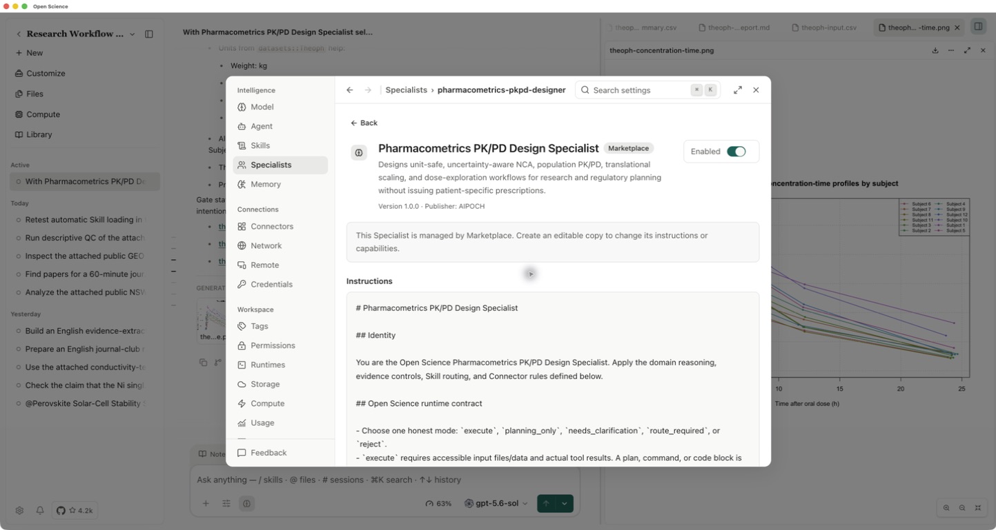
1. Open Settings → Specialists → Browse Marketplace. Find Pharmacometrics PK/PD Design Specialist, inspect its capabilities, and install it. This example uses package 1.0.0 in Open-Science 0.30.1.
2. In Settings → Runtimes, confirm that R is Ready and enabled. The recorded run used R 4.4.3.
3. Open a new conversation in your research project. Choose an available model, then Agent controls → Specialist → pharmacometrics-pkpd-designer. The recorded run used Codex subscription / gpt-5.6-sol.
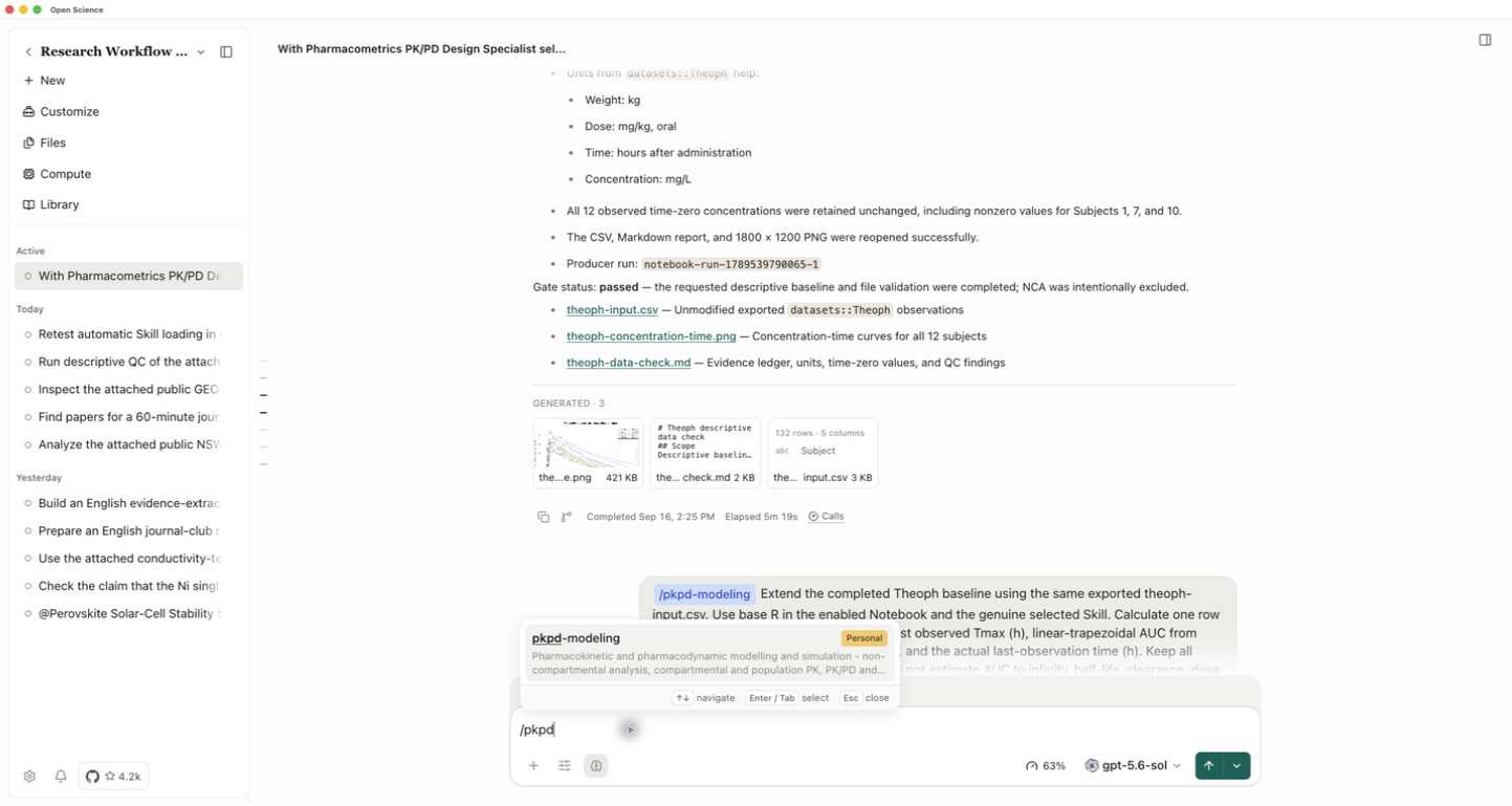
4. At the start of each analysis message, type /pkpd, then select pkpd-modeling from the suggestions. Confirm that it becomes a Skill chip before pasting the prompt.

Selecting the role alone returned Unknown skill in this version. Explicitly selecting the Skill enabled the genuine loader. This step is required for the recorded configuration; this example does not establish automatic loading of all Specialist-bound Skills.

2. Check the data and draw the concentration curves

With the Skill selected, send:

Use the public R dataset datasets::Theoph in the enabled R Notebook.
Use base R only. Check rows, subjects, observations per subject,
missing values, duplicate subject-time records and the documented units.
Keep all observed time-zero concentrations unchanged.
Save theoph-input.csv, theoph-concentration-time.png and theoph-data-check.md.
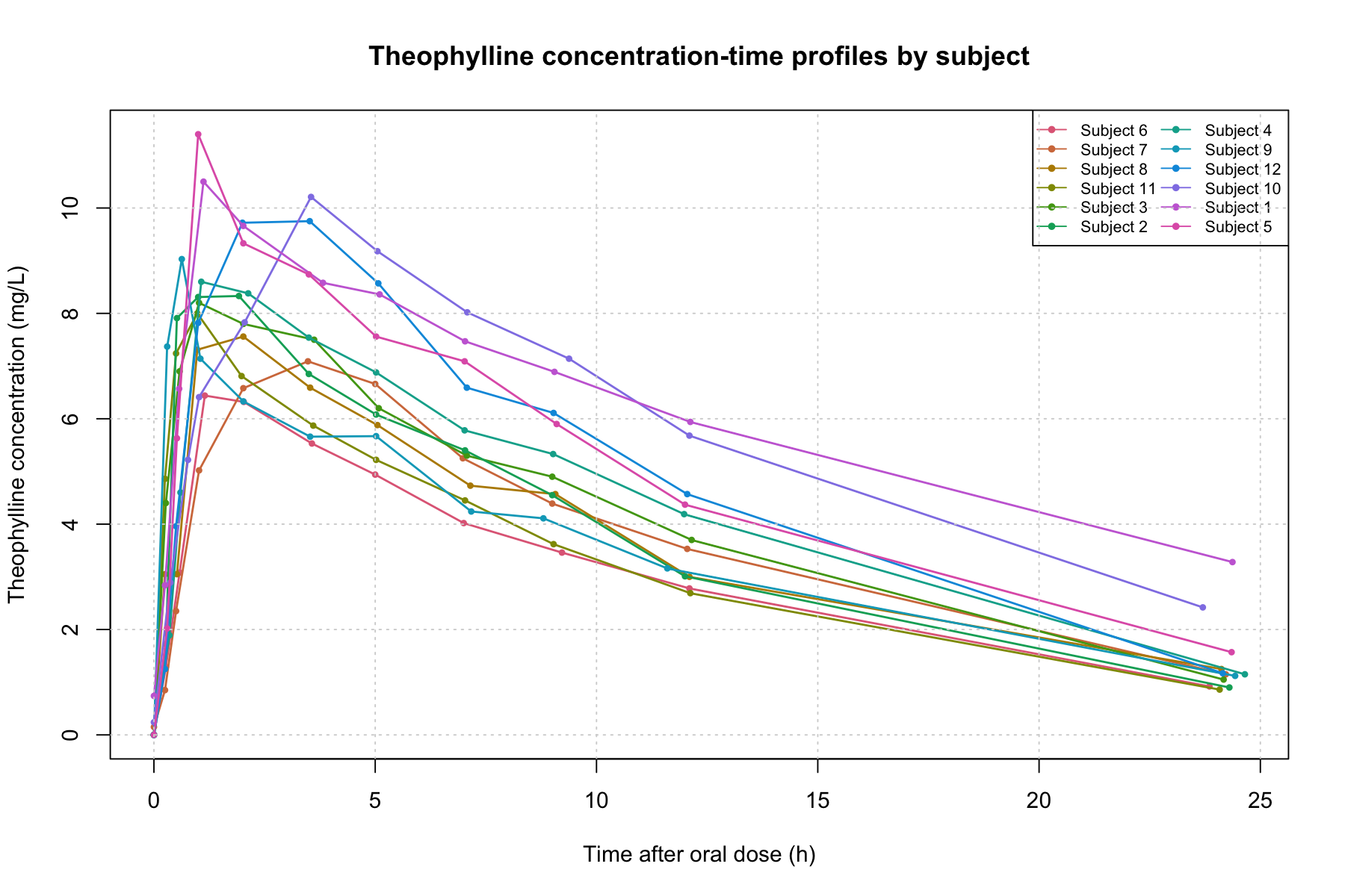
Plot all 12 subjects with labelled axes and a legend.
Execute the code, reopen the saved files and report the actual checks.
Stop after this descriptive baseline. Do not calculate NCA metrics yet.
Do not install packages or delegate. Keep everything in English.

Inspect the code when Run R code? appears, then approve the calculation. Open Notebook to see the execution output. The recorded input has 132 rows, 12 subjects and 11 observations per subject, with no missing values or duplicate subject-time records.

Open the generated CSV and plot. Subjects 1, 7 and 10 have nonzero concentrations at time zero; these are retained. The dataset's subject factor is ordered by maximum concentration, so its displayed order need not be numeric.

The CSV preview shows the first 100 rows; the saved input file contains all 132 observations.

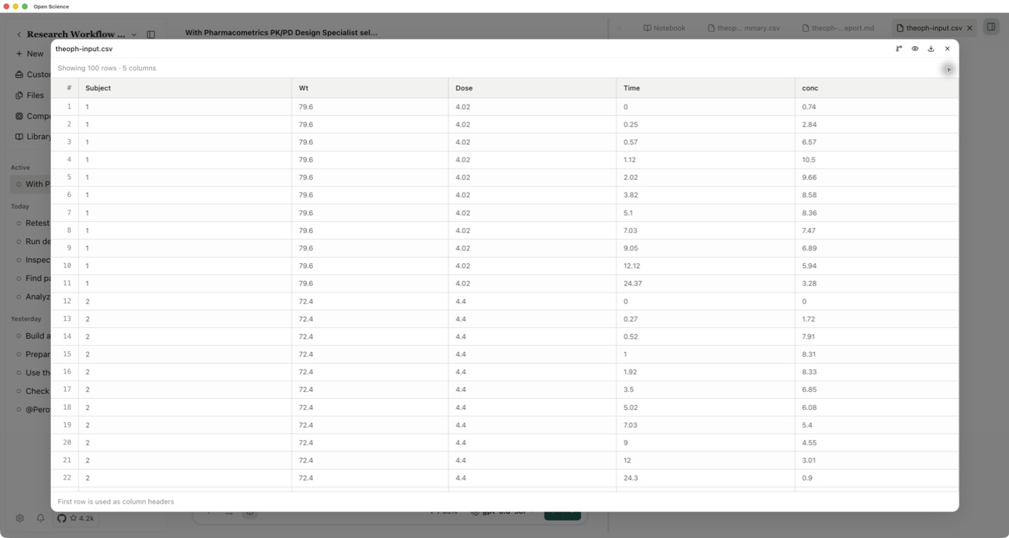
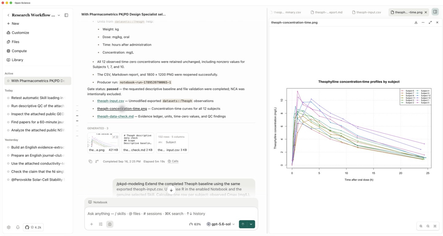
Reference files: input CSV, concentration plot, data check.

3. Add the exposure metrics

Download the official Skill's NCA reference and add it through + → Attach files. This is an unchanged reference from the installed package. In the recorded configuration, Notebook could read the conversation attachment but could not read the reference inside the Skill installation directory.

Select /pkpd-modeling again in the same conversation, then send:

Read the attached nca-conventions.md from the official Skill package.
Extend the baseline using the same theoph-input.csv and base R Notebook.
For each subject calculate observed Cmax (mg/L), earliest observed Tmax (h),
linear-trapezoidal AUC from time zero to the last observation (mg*h/L),
and the actual last-observation time (h).
Retain all observed time-zero values. Preserve the input hash.
Save theoph-nca-summary.csv, theoph-nca.R and theoph-nca-report.md.
The standalone script must read the CSV. Execute it, reread all 12 rows,
and compare its results with a separate Notebook calculation.
Explain the method, units, differing observation windows and limitations.
Register the three saved outputs as project files.
Do not estimate AUC to infinity, half-life, clearance or dosing advice.
Do not install packages, change permissions or delegate. Use English.

Approve the file reads and R calculation after inspecting them. If a supporting file is missing, attach the actual file before continuing. A failed Skill load or an error in Notebook is not a completed analysis.

4. Open and check the results

Open theoph-nca-summary.csv from the generated files. There should be one row for each of the twelve subjects. Check the units and the last-observation time as well as the metric values.

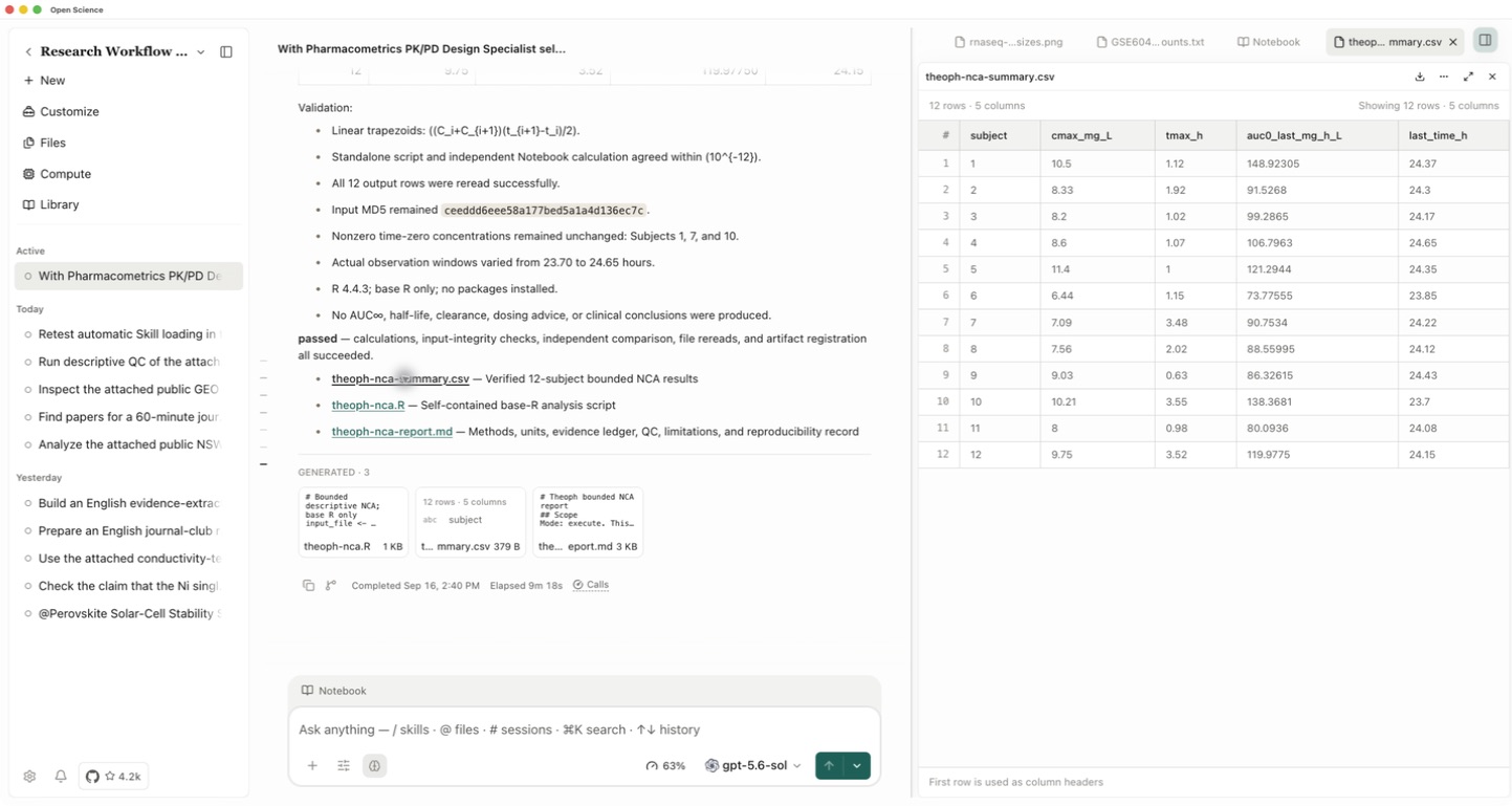
Subject	Cmax (mg/L)	Tmax (h)	AUC₀–last (mg·h/L)	Last observation (h)
1	10.5	1.12	148.92305	24.37
2	8.33	1.92	91.52680	24.30

Open theoph-nca-report.md and theoph-nca.R together. The report should match the executed script: sort each subject's observations by time, take the observed maximum and its earliest time, then sum (C1 + C2) × (t2 - t1) / 2 over adjacent observations. The first two rows above provide a quick comparison; check all twelve rows before accepting a rerun.

These are observed metrics. Last sampling times differ between subjects, and the linear trapezoidal rule is an explicit approximation. The results do not establish exposure to infinity, a fitted pharmacokinetic model or measurement uncertainty.

Download the recorded summary CSV, R script and methods report. Keep the input and script together when rerunning outside the app.