Check a regression result with a public dataset

Worked example Earnings after a job-training experiment

You have a small economic dataset and want to know whether a result changes when baseline characteristics are included. This example runs an unadjusted comparison and a prespecified adjusted regression, then saves the estimates and their uncertainty.

Deliverable: a Notebook calculation, a coefficient CSV and an English report. It uses the 445-observation experimental sample in jtrain2, attributed to LaLonde's National Supported Work analysis by the wooldridge data dictionary.

Prepare and attach the data

1. Download jtrain2.csv from Rdatasets and read the variable definitions in the dictionary.
2. Create a project and confirm that a Python runtime is enabled. This example uses pandas and statsmodels; install missing packages in the selected environment when needed.
3. Open a conversation, select a working model, then choose + → Attach files and select the CSV. Confirm the attachment appears before sending.

The outcome re78 and baseline variables re74 and re75 are real earnings in thousands of dollars. They refer to earnings in 1978, 1974 and 1975 respectively. Zero earnings are valid observations. train identifies training assignment; mostrn describes months of training and is not a baseline adjustment variable.

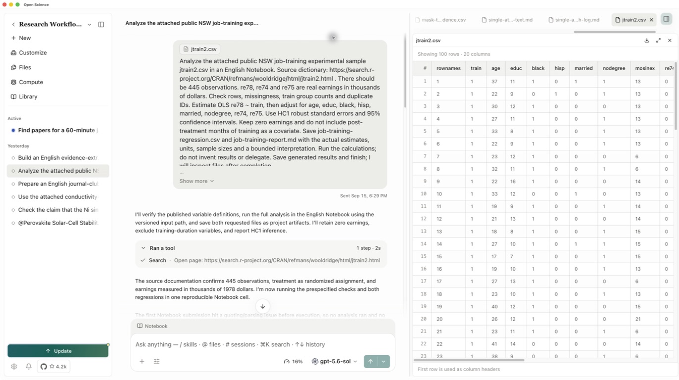
Click the attached CSV to preview it before sending the calculation request. Check train, re78, re74 and re75, including rows with zero earnings. The preview may show only 100 rows; the Notebook must count the entire file.

Run the prespecified comparison

Analyze the attached jtrain2.csv in an English Notebook.
Check row count, missingness, train group counts and duplicate IDs.
Estimate OLS re78 ~ train, then adjust for age, educ, black, hisp,
married, nodegree, re74 and re75. Use HC1 robust standard errors
and 95% confidence intervals. Keep zero earnings. Do not include
post-treatment months of training as a covariate.
Save job-training-regression.csv and job-training-report.md with
the estimates, units, sample sizes and a bounded interpretation.
Run the calculations; do not invent results or delegate.

Review the requested code when approval appears. It should read the attached CSV, fit the two specified models and save the outputs. Open Notebook to inspect the actual execution result. If execution fails, resolve the displayed error before treating any prose as a calculated result.

In the conversation, choose Notebook, open the executed Python cell and inspect its output. Look for the row and group counts before the regression summary. If the attached version cannot be resolved, ask the Agent to read the file mounted from this conversation’s attachment and retry; a failed cell is not a result. Keep the successful cell and its output with the saved files.

Inspect the saved result

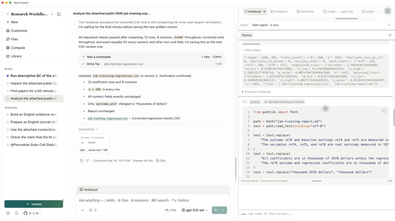
The example completed with 445 rows, 185 assigned to training, 260 controls, no missing values and no duplicate row identifiers. Both regressions retained all 445 observations.

Model	Training coefficient	HC1 standard error	95% confidence interval
Unadjusted	1.794	0.671	0.480 to 3.109
Adjusted for baseline variables	1.676	0.677	0.350 to 3.003

Coefficients and intervals are in thousands of dollars. These are results of this example's calculation, not quoted estimates from the original paper.

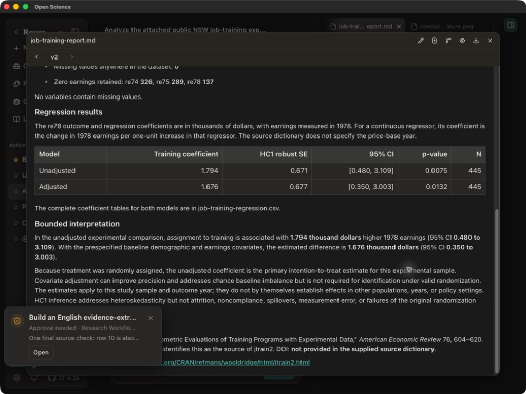
Open both generated files after the response completes. Compare the train rows in the CSV with the report and Notebook. You can download this run's coefficient table and report.

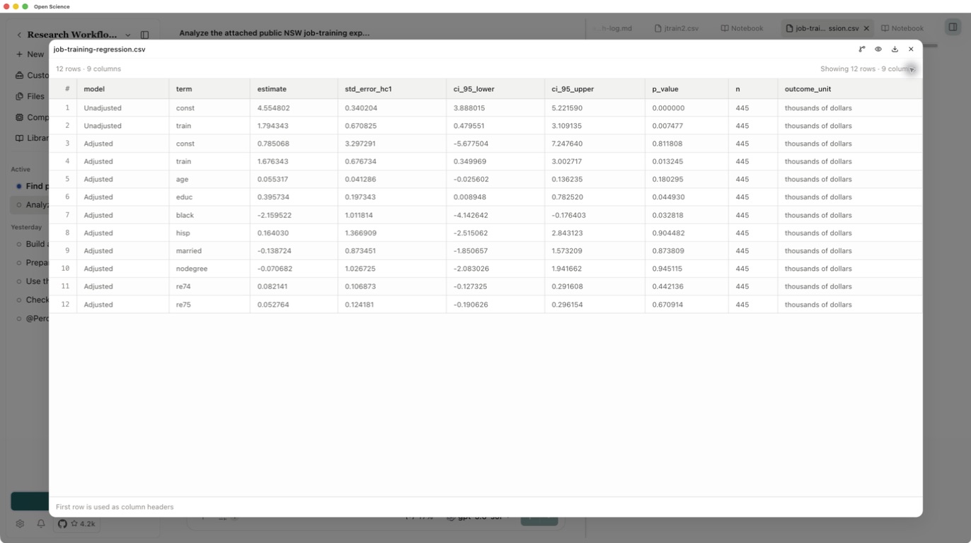
In Generated, open the CSV and expand its preview. The saved coefficient table has 12 rows · 9 columns: two rows for the unadjusted model and ten for the adjusted model. Locate each model’s train row and compare its estimate, robust standard error, interval, n and unit. Do not add an inflation base year that the source dictionary does not state. Use the preview’s Download button to keep the checked version.

Decide what the comparison supports

Baseline adjustment changes the estimate from about 1.79 to 1.68 thousand dollars. That is a sensitivity check for these two specifications. It does not establish robustness to every modelling choice or generalize the experiment to other populations and years. HC1 standard errors address heteroskedasticity; they do not repair problems in the original study design.

To hand the analysis to a colleague, retain the original CSV, variable dictionary, code and selected environment. Use Reproducibility checks to assess what is available for a later rerun.