Make a traceable figure with error bars

Worked example Temperature and electrical conductivity

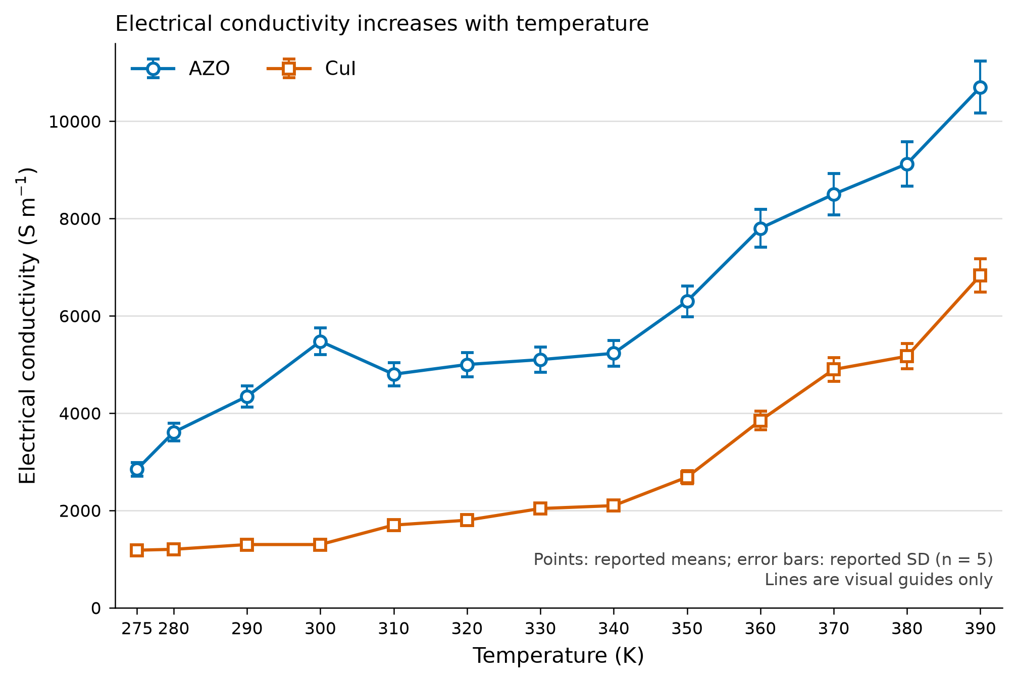
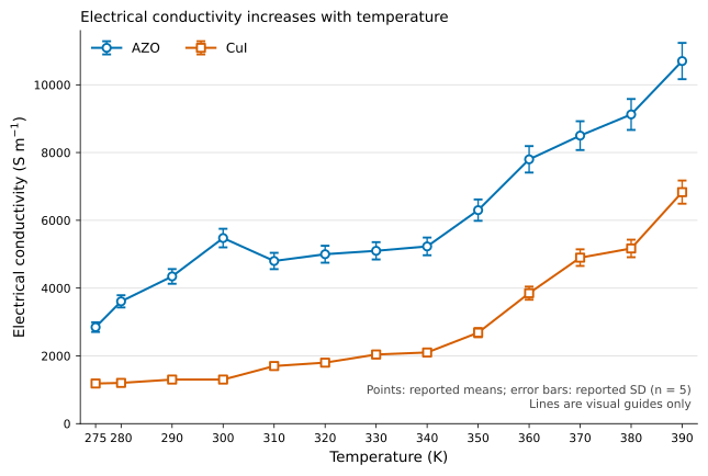
You need a scientific figure whose plotted points and uncertainty can be traced back to a data table. This example plots electrical conductivity for aluminium-doped zinc oxide (AZO) and copper iodide (CuI), keeping the publisher's reported standard deviations.

Deliverable: an English PNG and SVG, the plotted CSV, and a short methods file. The example uses published data, not a newly conducted experiment.

Prepare the data and its meaning

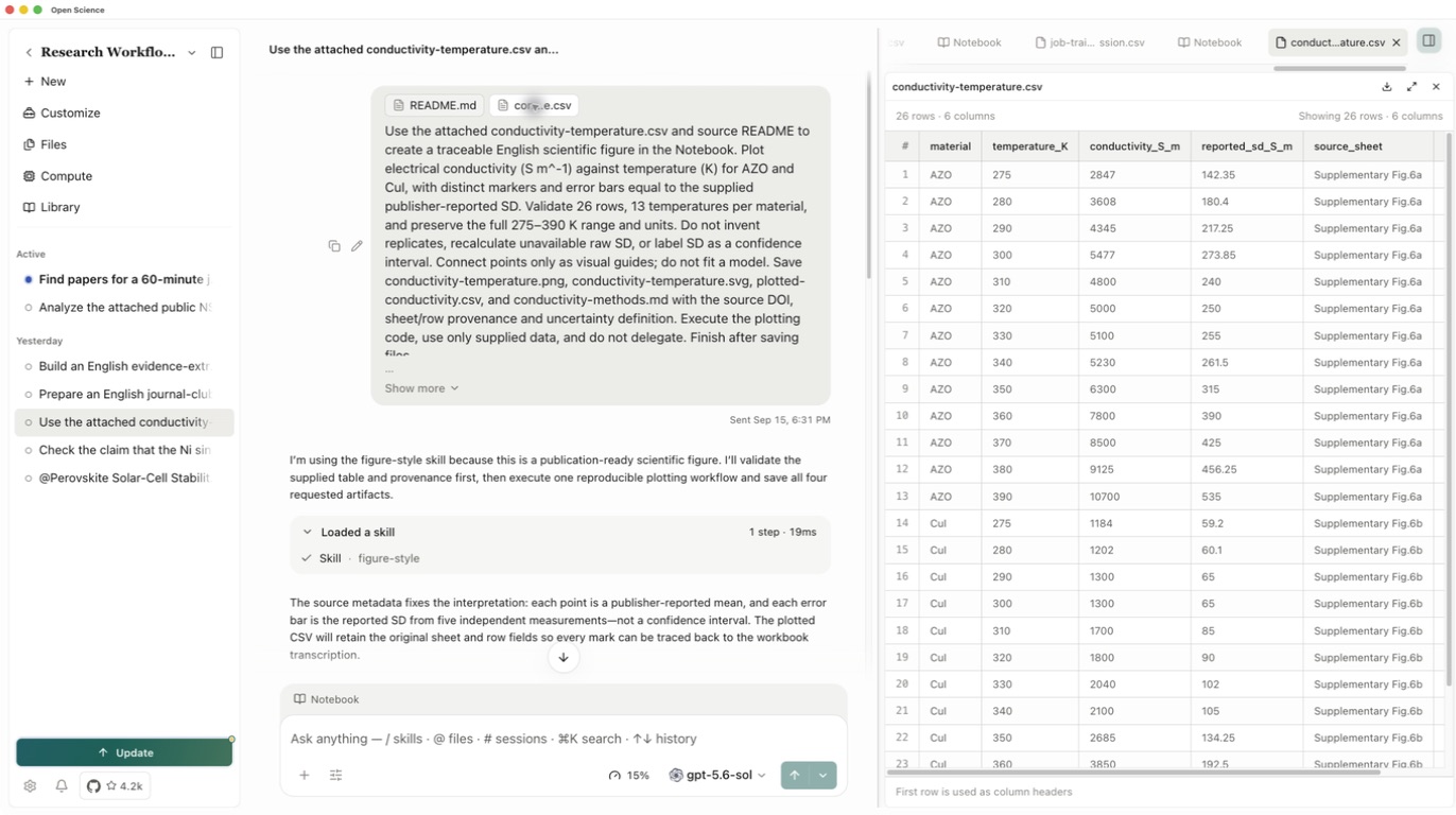
The source paper provides a Source Data workbook. The example CSV transcribes columns A, D and E from Supplementary Fig.6a and Supplementary Fig.6b, rows 3–15: temperature, electrical conductivity and reported SD. It contains 13 temperatures per material, covering 275–390 K.

Download the prepared CSV and source notes. The CSV retains the original sheet and row for every point. The paper describes SD from five measurements per temperature; individual replicate measurements are not supplied in these columns, so this workflow does not recalculate SD.

1. Create a project with a working model and an enabled Python runtime.
2. Open a conversation and attach both files using + → Attach files.
3. Confirm the numerical columns and units before plotting: K for temperature and S m⁻¹ for conductivity and its SD.

Click the attached CSV to open the preview. It should show 26 rows · 6 columns, including material, temperature, conductivity, SD and source sheet/row. Open the source note too; the captured run used the filename README.md for the note supplied here as conductivity-source.md.

Ask for the figure and the data behind it

Use the attached conductivity CSV and source notes to create a figure
in the Notebook. Plot electrical conductivity (S m^-1) against
temperature (K) for AZO and CuI. Use distinct markers and error bars
equal to the supplied publisher-reported SD.
Check 26 rows, 13 temperatures per material, and the 275–390 K range.
Do not invent replicates or label SD as a confidence interval.
Connect points only as guides; do not fit a model.
Save conductivity-temperature.png, conductivity-temperature.svg,
plotted-conductivity.csv and conductivity-methods.md.
Keep all labels and notes in English. Execute the code and save files.

Review any code or package request, then inspect the actual Notebook result. A chart described in the answer is not yet a saved figure.

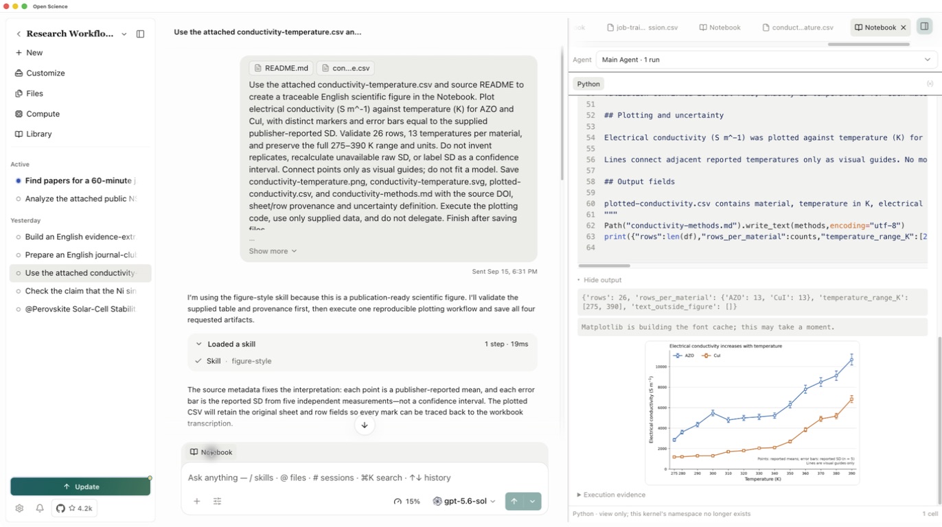
Choose Notebook in the conversation. Open the completed Python cell and inspect its output: 26 total rows, 13 rows for each material, the 275–390 K range and the plotted figure. If input resolution fails, have the Agent use the CSV attached to this conversation, then verify a successful execution before continuing.

Check the figure and export

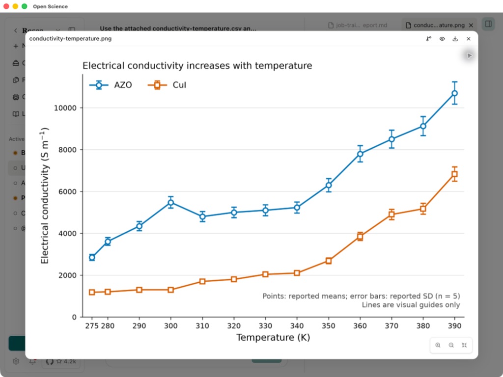
Open the generated PNG. Confirm that both materials are distinguishable, the endpoints are visible, the axes state units and the uncertainty note says reported SD. The lines only connect measurements; the dip in AZO conductivity after 300 K remains visible.

Open plotted-conductivity.csv and compare it with the input. In this run all 26 rows preserved the temperatures, conductivity values, SDs and source sheet/row identities. Open conductivity-methods.md to check the source DOI and uncertainty definition.

The Generated area should contain four files. Open the methods file and use the download icon in each preview to save the version you checked. If one output is missing, request that specific file and reopen it; a successful PNG does not prove the SVG or data table was saved.

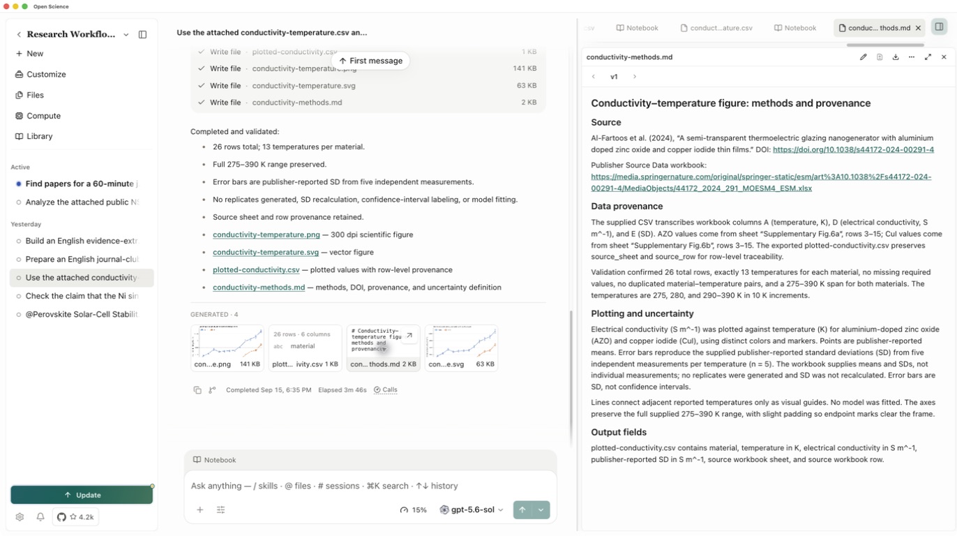
Use PNG for quick sharing and SVG where vector artwork is useful. This run's PNG, SVG, plotted data and methods are available for comparison.

For your own measurements, decide whether error bars should show SD, standard error or a confidence interval before asking for a plot. Give the agent the required raw measurements or already calculated uncertainty, together with its definition. Keep missing uncertainty explicit.