Scientific tools

Run a scientific calculation only after its actual input and execution environment are clear. Choose a local Notebook, a Connector or an external runner according to the method and its dependencies.

Choose where the calculation runs

Route	Suitable work	Readiness check
Python Session Notebook	Data parsing, numerical summaries and plotting	Bound Python runtime and installed packages
R Session Notebook	R analysis and packages	Enabled R runtime bound to this session
Built-in Connector	Database retrieval or supported deterministic operation	Connector available to the agent, credentials/network as required
Remote Compute	Host-specific software, GPU or batch jobs	Eligible enabled host, environment and scheduler

A shell command is not interchangeable with a Session Notebook run: their runtime, mounted inputs and provenance can differ. Request the intended route explicitly.

Packages and dependencies

Step	What to do	Successful result
Inspect	Ask for inspect_packages in the intended language/runtime	Installed/missing status and versions
Install	Use the supported manage_packages flow for the bound environment	Completed installer output, not only “installation started”
Restart	Restart/rebind the kernel if the app requests it	The next cell uses the updated environment
Verify	Import the package in that same Notebook	Actual version and a small working operation

If package installation returns HTTP CONNECT 403, check the affected package hostname and Network settings before retrying. Use an existing package only when it supports the method you need; a successful calculation does not mean a failed package installation was repaired.

Execute and verify a local RNA-seq calculation

Worked example Check sample-level counts in the GSE60450 matrix

1. Attach the GSE60450 input.
2. Select the Python or R Notebook runtime. Inspect its version before installing anything.
3. Ask for full-matrix dimension and count-integrity checks; exclude EntrezGeneID and Length from the sample columns.
4. Calculate total counts, zero-count genes, detected genes and median among detected genes for each full sample ID.
5. Save new CSV, chart and methods report. Keep the source unchanged and compare its SHA-256 before/after.
6. Reopen all outputs. Cross-check sample count, labels and values; inspect the actual Notebook code and logs.

Compare output identifiers and metrics with the example baseline. Keep the raw input unchanged. Descriptive counts do not establish normalized expression, differential expression or a clinical conclusion.

Python QC CSV · R/Python comparison · Skill validation.

Design a small protein sequence on CPU

Worked example Design candidate sequences for the 1UBQ backbone

This route runs the official ProteinMPNN CLI on human ubiquitin, PDB 1UBQ chain A. It creates one candidate each with the vanilla and soluble checkpoints. It is an inverse-folding calculation conditioned on an existing backbone.

Prepare the runner and weights

Use a supported Python with working venv and pip, Git, internet access and a writable folder. The following commands are for macOS/Linux shells. On Windows use the corresponding .venv\Scripts\python.exe and set CUDA_VISIBLE_DEVICES using your shell's syntax.

mkdir protein-design
cd protein-design
git clone https://github.com/dauparas/ProteinMPNN.git
git -C ProteinMPNN checkout 8907e6671bfbfc92303b5f79c4b5e6ce47cdef57
python3 -m venv .venv
.venv/bin/python -m pip install torch numpy
.venv/bin/python -c "import sys, torch, numpy; print(sys.version); print(torch.__version__, numpy.__version__)"
.venv/bin/python -m pip freeze > environment.txt

The pinned checkout includes vanilla_model_weights/v_48_020.pt and soluble_model_weights/v_48_020.pt; confirm both files exist. Download the 1UBQ input into protein-design as 1UBQ.pdb. Keep the sequence input separate from output folders.

This setup installs packages in an external virtual environment. If pip reports no compatible distribution, choose a Python version supported by the available PyTorch wheel before retrying. Record environment.txt; changing Python, PyTorch or NumPy may change numerical output. If an old virtual environment no longer finds its base interpreter after a system update, recreate it with the current compatible Python.

Run both models and save their outputs

From protein-design, run:

CUDA_VISIBLE_DEVICES="" .venv/bin/python ProteinMPNN/protein_mpnn_run.py \
  --pdb_path 1UBQ.pdb --pdb_path_chains A --model_name v_48_020 \
  --num_seq_per_target 1 --batch_size 1 --sampling_temp 0.1 --seed 42 \
  --out_folder outputs/vanilla
CUDA_VISIBLE_DEVICES="" .venv/bin/python ProteinMPNN/protein_mpnn_run.py \
  --pdb_path 1UBQ.pdb --pdb_path_chains A --model_name v_48_020 \
  --use_soluble_model --num_seq_per_target 1 --batch_size 1 \
  --sampling_temp 0.1 --seed 42 --out_folder outputs/soluble

Both commands use chain A, one sequence, temperature 0.1 and seed 42. Clearing CUDA device visibility makes this runner use CPU. Expect outputs/vanilla/seqs/1UBQ.fa and outputs/soluble/seqs/1UBQ.fa; keep their names separate when importing or publishing them.

To execute through Open-Science, grant the prepared folder using Your files → Grant folder…, then ask the agent to run these commands with the environment's absolute Python path and that working directory. Inspect the command and scope at approval. Ask it to publish the two FASTAs and a comparison report, then reopen all three in Files. A file left only in the working directory still needs publication.

Skill package loading

If the built-in model Skill fails package path validation, report that error through Troubleshooting. The CLI route above remains a separate method; successful CLI execution does not establish that native Skill loading works.

Check the designed sequences

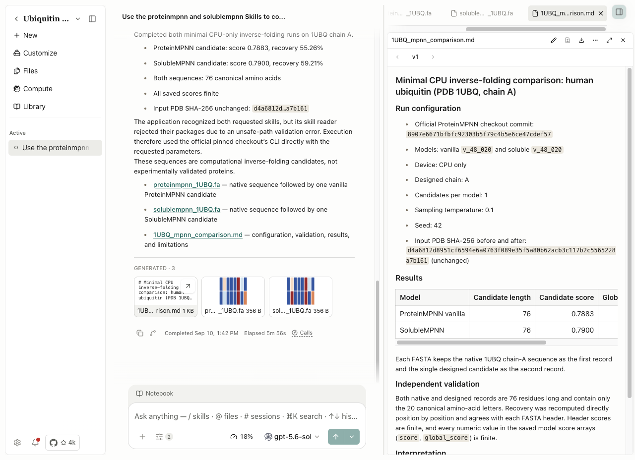
The saved outputs in this example contained the following results:

Output	Designed residues	Score	Recovery against native
ProteinMPNN FASTA	76	0.7883	55.26%
SolubleMPNN FASTA	76	0.7900	59.21%

Each FASTA contains two records: the native sequence first, then the single designed candidate. Independent checks confirmed canonical amino acids, 76 residues per record, finite scores, directly recomputed recovery and unchanged PDB SHA-256. Saved artifact bytes matched the runner outputs. The comparison report records settings and limitations. Scores from this one-candidate comparison do not establish which model yields better folding, solubility or function.

Diagnose by the failing stage

Symptom	Next check
No runtime / R unavailable	Install or enable the interpreter through Runtimes, then bind it.
ImportError / ModuleNotFoundError / no package called	Inspect the selected environment and use managed package installation.
Unknown Skill / invalid kernel helper	Distinguish a method package from an actual callable Notebook helper.
Input version unavailable / file not found	Resolve the exact current input through the application; do not guess a path.
Network/HTTP failure	Keep host, operation and actual status; use network controls and error guidance.
Output exists only in a working directory	Publish it through the supported artifact route and reopen the saved version.
No producer block / partial environment	Retain the limitation; do not manufacture missing evidence.

For remote jobs, inspect host readiness, submission, status and harvested output separately. The Direct SSH RNA-seq example completed and its outputs were independently checked. Slurm terminal monitoring requires readable accounting. The same chapter now documents a verified A100 ProteinMPNN run with an isolated CUDA environment and independent output checks. CPU-capable methods remain separately assessable.

For supported long-running work, follow Background tasks and result delivery. Inspect the actual run and saved outputs after delivery. Environment & Packages, Compute Environment Setup and Remote Compute (SSH) stay enabled, but their runtime, network and host requirements still apply.

Implementation reference: notebook.ts, SKILL.md, SKILL.md.